Hi! I’m Peter!
Blog
-
An M.C. Escher-inspired poster
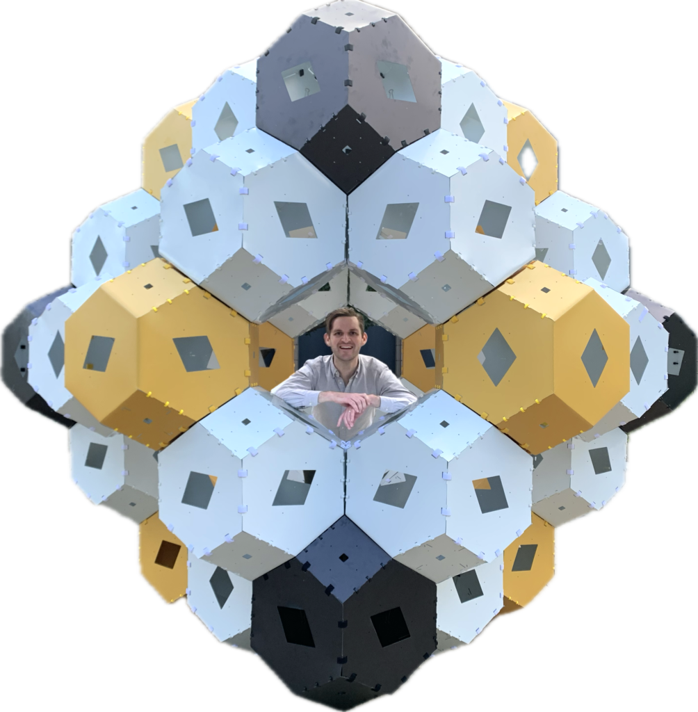
I wanted an excuse to use Harvey Mudd’s large format printer, so I made a movie-sized (27″×40″) poster for my office based on the second term of OEIS sequence A368138(n): \(A368138(2) = 154\). The idea here is that you have a a collection of tiles like
 , which you can rotate and mirror; you then choose a \(n \times n\) grid of these tiles, and repeat that pattern infinitely over the plane. I recently learned that this particular example (for \(n = 2\)) was first enumerated in a 1996 paper by Dan Davis, On a Tiling Scheme from M. C. Escher, in The Electronic Journal of Combinatorics.
In my paper, “Counting Tilings of the \(n \times m\) Grid, Cylinder, and Torus,” we give a method for counting these kinds of problems in full generality. While revising the paper, I learned from Doris Schattschneider’s 1990 book Visions of Symmetry (pp 44-48) that the artist M.C. Escher was perhaps the first person to attempt counting this. (In particular, Escher successfully enumerated A368145(2) = 23.)

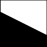
Figure 3 from Bill Keehn’s and my paper “Counting Tilings of the \(n \times m\) Grid, Cylinder, and Torus“, which illustrates that there are many equivalent choices when repeating a \(2 \times 2\) pattern when ignoring the boundary. Notice how the whitespace and the black space are \(180^\circ\) rotations of each other. Ami Radunskaya pointed out to me that this looks like “op art.”
If you had to choose one of these patterns to tile your bathroom floor, which would you pick?
-
Triangle Center Patterns
I made a video that illustrates a particularly interesting “discrete state random dynamical system,” which was inspired by a Tweet (and a mistake) that I saw.
First, be hypnotized by this video, which I recommend you watch in 4K, and then scroll down to read about the inspiration and the cool math going on under the hood.
Matt Henderson’s tweet
This whole exploration came from a “happy accident” that Matt Henderson made (and corrected) in the Tweets below. Watch the video in the first tweet, which shows an concrete example of the “discrete state random dynamical system” that I mentioned earlier.
Matt’s mistake got me interested! If the centroid and the incenter create such interesting and intricate designs, what about other triangle centers like the circumcenter or the orthocenter? In particular, I was interested in finding examples of interesting triangle centers from Clark Kimberling’s Encyclopedia of Triangle Centers (ETC), which is a database with over 53,000 named triangle centers, including all of those that you have heard about.
Patterns from other triangle centers
Instead of illustrating the results of this process on hexagons as Matt did in his tweet, I’ve done the iterative process on squares. Here are six examples illustrating the patterns for various triangle centers from ETC.
Some basics of triangle centers
In the video at the top, I interpolate between 20 chosen triangle centers in a continuous way so that we can see how the image transforms as we transform the choice of triangle center.
In order to understand what’s going on, you have to understand something about coordinates. We can define a triangle center with a map \(f\colon \mathbb{R}^3 \to \mathbb{R}\) such that \(f(a,b,c)\) is symmetric in \(b\) and \(c\). What we do is take the triangle with vertices \(\vec{v}_1\), \(\vec{v}_2\), and \(\vec{v}_3\), define \(a = |\vec{v}_2 – \vec{v}_3|\), \(b = |\vec{v}_1 – \vec{v}_3|\), and \(c = |\vec{v}_1 – \vec{v}_2|\), and define the midpoint as the weighted average \[\frac{f(a,b,c) \vec{v}_1 + f(b,c,a)\vec{v}_2, + f(c,a,b)\vec{v}_3}{f(a,b,c) + f(b,c,a) + f(c,a,b)}.\] Whenever \(f(a,b,c)\), \(f(b,c,a)\), and \(f(c,a,b)\) are simultaneously positive, this will describe a point inside the triangle. This way of describing points in space is called a “barycentric coordinate system“.

An illustration of the vertices and sides. In the table below, I give examples of five triangle centers and their description in barycentric coordinates. In the case of \(X(2)\), the barycentric coodinates say that the centroid is just an honest average of the vertices. In all other cases, the other triangle centers are weighted averages of the vertices.
Triangle Center Barycentric X(1) = INCENTER \(f(a,b,c) = a\) X(2) = CENTROID \(f(a,b,c) = 1\) X(6) = SYMMEDIAN POINT \(f(a,b,c) = a^2\) X(10) = SPIEKER CENTER \(f(a,b,c) = b + c\) X(58) = ISOGONAL CONJUGATE OF X(10) \(\displaystyle f(a,b,c) = \frac{a^2}{b + c}\) A table of five triangle centers and the corresponding barycentric coordinates. A curve of triangle centers
The triangle centers in the video are all described by functions of the form \[f(a,b,c) = a^{x_1}(b + c – a)^{x_2} (bc)^{x_3} (b^{x_4} + c^{x_4})^{x_5},\] where \((x_1, x_2, x_3, x_4, x_5) \in \mathbb{R}^5\) and each frame follows a path in \(\mathbb{R}^5\), which intersects a triangle center from ETC for a single frame every ten seconds. In order to get this path in five-dimensional space, the code stitches together twenty piecewise-defined Bézier curves into a differentiable curve that goes through those twenty “anchor points”, as suggested by the following illustration. (Thankfully I could reuse some of the code I wrote for my Twitter bot @BotzierCurves!)

A two-dimensional example of a curve through seven anchor points. In addition to choosing a slightly different triangle center in each frame, the colors of the points change throughout time as well. For example, in the picture below, the pixel is colored white if the same side is chosen twice in a row, red if the opposite side is chosen, and blue or green if the side to the left or right of the previous side is chosen. In the video, these colors change too, by following a Bézier curve through the three-dimensional RGB colorspace.
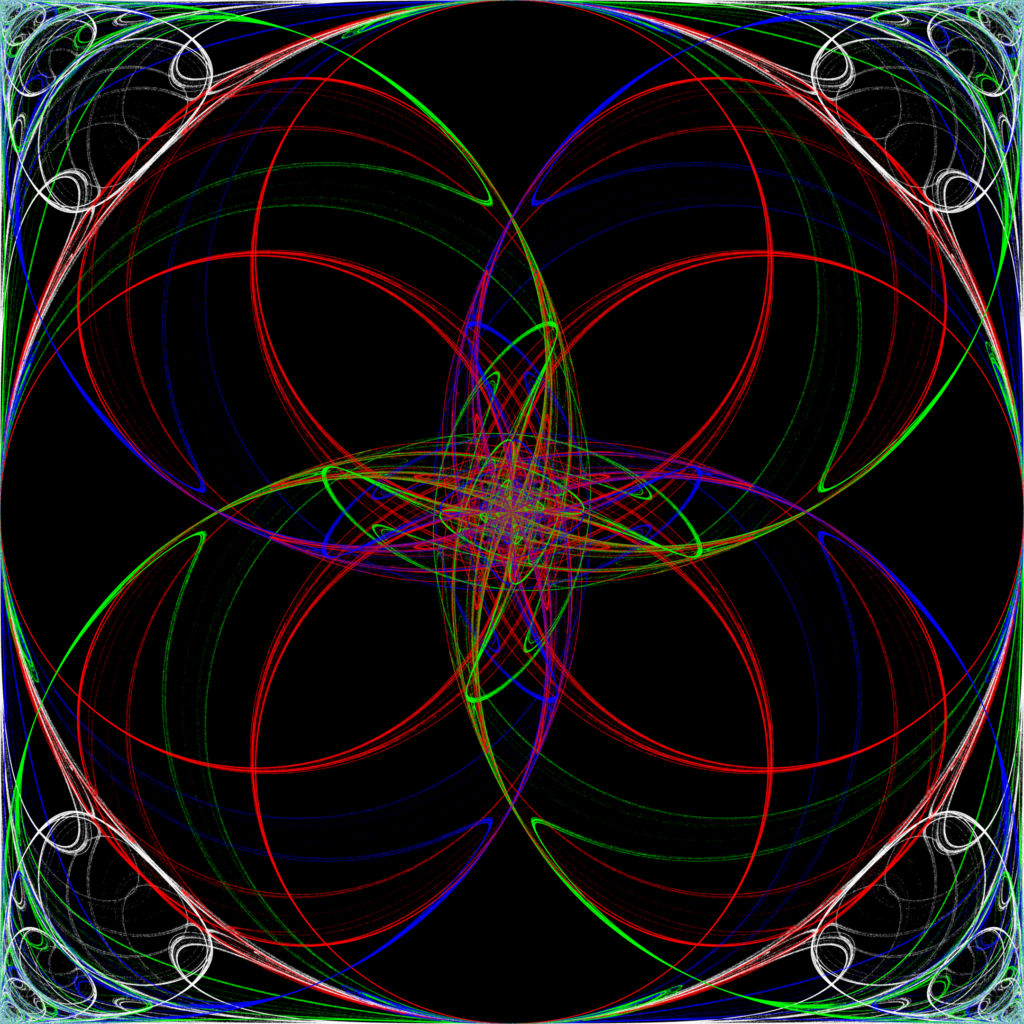
An illustration of a triangle center pattern where the color of the pixel depends on the order that the sides are chosen. You can download the code for yourself by visiting my MathArt repository on Github. If you have thoughts on this, if you want to play around with these ideas together, or if you just want to chat, please don’t hesitate to reach out!
-
How to Make Animated Math GIFs: LaTeX + TikZ
The first animated GIF that I ever made was made with the LaTeX package TikZ and the command line utility ImageMagick. In this post, I’ll give a quick example of how to make a simple GIF that works by layering images with transparent backgrounds on top of each other repeatedly.
TikZ code
In our first step toward making the above GIF, we’ll make a PDF where each frame contains one of the above circles on a transparent background. In this case, each circle is placed uniformly at random with its center in a \(10 \times 10\) box, with a radius in \([0,1]\), and whose color gets progressively more red and less green with a random amount of blue at each step.
\documentclass[tikz]{standalone}
\usepackage{tikz}

\begin{document}
\foreach \red[evaluate=\red as \green using {255 - \red}] in {0,1,...,255} {
  \begin{tikzpicture}
    \useasboundingbox (0,0) rectangle (10,10);
    \pgfmathrandominteger{\blue}{0}{255}
    \definecolor{myColor}{RGB}{\red,\green,\blue}
    \fill[myColor] ({10*random()},{10*random()}) circle ({1+random()});
  \end{tikzpicture}
}
\end{document}
Starting with
\documentclass[tikz]{standalone}says to make eachtikzpictureits own page in the resulting PDF.Next we loop through values of
\redfrom0to255, each time setting\greento be equal to255 - \redso that with each step the amount of red goes up and the amount of green goes down.The command
\useasboundingbox (0,0) rectangle (10,10);gives each frame a \(10 \times 10\) bounding box so that all of the frames are the same size and positioned the same way.The command
\pgfmathrandominteger{\blue}{0}{255}chooses a random blue values between0and255.The command
\fill[myColor] ({10*random()},{10*random()}) circle ({1+random()});places a circle with its center randomly chosen in the \(10 \times 10\) box and with a radius between \(1\) and \(2\).ImageMagick
When we compile this code, we get a PDF with one circle on each page. In order do turn this PDF into an animated GIF, we convert the PDF using ImageMagick, a powerful command-line utility for handling images. If we named our PDF
bubbles.pdfthen running the following command in the terminal (in the same directory asbubbles.pdf) will give us an animated GIF calledbubbles.gif.convert -density 300 -delay 8 -loop 0 -background white bubbles.pdf bubbles.gif
I hope that you use this blog post as a jumping off point for making animated GIFs of your own! If you do, please reach out to share them with me!


